A Deep Learning Vision Classifier built on Tensorflow to classify the provided image between ice cream 🍨 and pizza 🍕. This is a simple exercise to start with machine learning. You can check the app at: https://pizza-vs-icecream.streamlitapp.com/
In this project, we will be looking at the dataset journey(from gathering to preparation), and then will jump into the python code for creating the model, the FlaskAPI backend, and Streamlit python code.
Dataset
The dataset used is hosted on Kaggle, and the data was captured from Freepik using python script. Once the data was captured, Roboflow was used to organize and annotate. Roboflow can be used for more advanced features like augmentation, pre-processing, getting more examples, and exporting the data in different formats.
I exported the data in folder format which was able to give me the data in the below format:
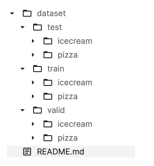
The dataset consists of around 1300 images. 718 images for training, 208 images for validation, and 106 images for testing.
Python Logic for Model Creation
The full code is accessible on GitHub through this link. But we will go over the important points in this article.
Import Library
import os
import math
import numpy as np
import matplotlib.pyplot as plt
import tensorflow as tf
import tensorflow_hub as hub
from tensorflow.keras import layers

print(tf.__version__)
Loading Data
We have loaded the data using ImageDataGenerator with multiple augmentation layers as our dataset is quite small, with only 718 images for training.
train_datagen = tf.keras.preprocessing.image.ImageDataGenerator(
    rescale=1./255,
    rotation_range=40,
    width_shift_range=0.2,
    height_shift_range=0.2,
    shear_range=0.2,
    zoom_range=0.2,
    fill_mode='nearest',
    horizontal_flip=True,
)

train_generator = train_datagen.flow_from_directory(
    TRAIN_DIR,
    target_size=(IMG_SIZE, IMG_SIZE),
    batch_size=BATCH_SIZE,
    class_mode='sparse'
)
Found 718 images belonging to 2 classes.
val_datagen = tf.keras.preprocessing.image.ImageDataGenerator(
    rescale=1./255
)

val_generator = val_datagen.flow_from_directory(
    VAL_DIR,
    target_size=(IMG_SIZE, IMG_SIZE),
    batch_size=BATCH_SIZE,
    class_mode='sparse'
)
Found 208 images belonging to 2 classes.
test_datagen = tf.keras.preprocessing.image.ImageDataGenerator(
    rescale=1./255
)

test_generator = test_datagen.flow_from_directory(
    TEST_DIR,
    target_size=(IMG_SIZE, IMG_SIZE),
    batch_size=BATCH_SIZE,
    class_mode='sparse'
)
Found 106 images belonging to 2 classes.
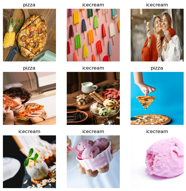
Data Visualization
show_examples(train_generator)
IMAGE SHAPE: (480, 480, 3)
Now let’s jump over the model architecture and see how we smartly used the pre-trained model as a feature extractor.
Model Architecture
FEATURE_EXTRACTOR_URL = 'https://tfhub.dev/google/imagenet/efficientnet_v2_imagenet21k_ft1k_m/feature_vector/2'

model = tf.keras.Sequential([
    hub.KerasLayer(FEATURE_EXTRACTOR_URL, trainable=False, input_shape=(IMG_SIZE, IMG_SIZE, 3)),
    layers.Dense(2, activation='softmax')
])

model.summary()

model.compile(
    optimizer='adam',
    loss='sparse_categorical_crossentropy',
    metrics=['accuracy']
)
Model: "sequential"
_________________________________________________________________
 Layer (type)                Output Shape              Param #
=================================================================
 keras_layer (KerasLayer)    (None, 1280)              53150388

 dense (Dense)               (None, 2)                 2562

=================================================================
Total params: 53,152,950
Trainable params: 2,562
Non-trainable params: 53,150,388
_________________________________________________________________
As we have fewer training images with drastic differences b/w images such as color, size, people, placement & amount of target items, it is a quite time-consuming and complex task to train the model from scratch. That’s why it’s a best practice to check if a pre-trained model can be utilized.
After multiple iterations of custom model architecture, we have used the ‘EfficientNet V2’ model from TensorFlow Hub which was trained on imagenet-21k (Full ImageNet, Fall 2011 release) and fine-tuned on ImageNet1K as a feature extractor and a single dense layer which is used as output layer having 2 nodes defining 2 classes in the dataset.
Model Training
SAVED_MODEL_PATH = './models/pizza_vs_icecream_model.h5'

model_checkpoint = tf.keras.callbacks.ModelCheckpoint(
    SAVED_MODEL_PATH,
    monitor='val_loss',
    save_best_only=True
)

early_stopping = tf.keras.callbacks.EarlyStopping(
    monitor='val_loss',
    patience=5
)

history = model.fit(
    train_generator,
    steps_per_epoch=len(train_generator),
    epochs=50,
    validation_data=val_generator,
    validation_steps=len(val_generator),
    callbacks=[model_checkpoint, early_stopping],
    verbose=2
)
Epoch 1/50
23/23 - 52s - loss: 0.3017 - accuracy: 0.8900 - val_loss: 0.0705 - val_accuracy: 0.9952 - 52s/epoch - 2s/step
Epoch 2/50
23/23 - 35s - loss: 0.0480 - accuracy: 0.9903 - val_loss: 0.0363 - val_accuracy: 0.9952 - 35s/epoch - 2s/step
Epoch 3/50
23/23 - 35s - loss: 0.0348 - accuracy: 0.9889 - val_loss: 0.0221 - val_accuracy: 1.0000 - 35s/epoch - 2s/step
.
.
.
Epoch 38/50
23/23 - 34s - loss: 0.0015 - accuracy: 1.0000 - val_loss: 0.0031 - val_accuracy: 1.0000 - 34s/epoch - 1s/step
Epoch 39/50
23/23 - 34s - loss: 0.0064 - accuracy: 0.9972 - val_loss: 0.0024 - val_accuracy: 1.0000 - 34s/epoch - 1s/step
Epoch 40/50
23/23 - 34s - loss: 0.0050 - accuracy: 0.9972 - val_loss: 0.0027 - val_accuracy: 1.0000 - 34s/epoch - 1s/step
And, definitely in our use case, the pre-trained model has worked wonderfully. Let’s finally evaluate the model.
Model Evaluation
saved_model = tf.keras.models.load_model(
    SAVED_MODEL_PATH,
    custom_objects={'KerasLayer': hub.KerasLayer}
)

saved_model.evaluate(test_generator)
4/4 [==============================] - 7s 1s/step - loss: 0.0043 - accuracy: 1.0000
Out[15]:
[0.004329057410359383, 1.0]
As the model is working flawlessly even on the test data which the model has never seen, it’s time to take this model to production. Upload the saved model to Google Cloud, which will be used in the next section for building the backend services.
Flask API Backend Code
Python code for Flask API is straightforward and the detailed code can be accessible at main.py. We load the saved(Google Cloud) TensorFlow model once the Flask run initially and we get the POST request at the root level along with the image and first thing will be, pre-processing the received image.
The pre-processing steps include:
- Decoding the base64 image
- Reading the image using
tf.io.decode_image(image, channels=3) - Resizing the image to match the image size used to train the model i.e., 480
- Converting the image to array
- And finally, normalize the image array by dividing it with 255.0
After pre-processing, we ran the input image array through the model using model.predict(input) and get the output as probability of classes. Using this the high-probability class is identified and returned.
Front-End Streamlit App
To make the model easier to use, let’s build a Streamlit App, which provides astonishing UI with little python code. The code is accessible at app.py.
The purpose of this python code is to provide the upload facility to users, so they can upload an image that will be encoded and sent to the Flask API for prediction. Once the result is returned from the API request, using Streamlit functions, we can show the result in very beautiful formats along with the uploaded images.
Final Connections b/w Streamlit and Flask API
The whole code was uploaded to GitHub and the Flask API code was uploaded to the Google Cloud Run functionality and the Streamlit app code was connected to the Streamlit app.
Results
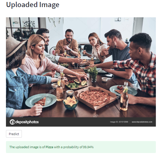
Result 1
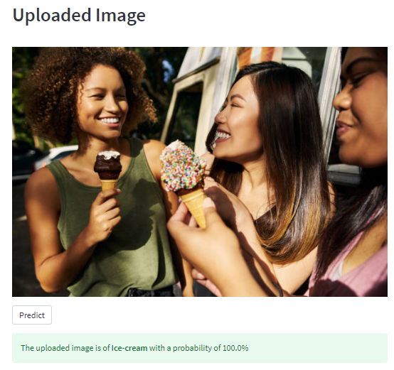
Result 2
Closing Note
This was a fun project for me as the binary classification task was simple, but if we look at the whole project in a nutshell from data collection to taking the model to production with beautiful UI, it was a challenging task too.
A great beginner-friendly project.